Fast Splat Viewing

FastGaussianRenderer is a forward-only rendering path for 3D Gaussian Splatting that trades autodiff support for speed: 1.5–2× faster than the training rasterizer on typical scenes and up to 3.7× when large splats cover many pixels — while matching it pixel-for-pixel (45+ dB PSNR on real scenes).

It adapts the ideas of fast-gaussian-rasterization (a CUDA/OpenGL geometry-shader pipeline) to Metal compute kernels and MLX's lazy graphs. Use it anywhere you only need images: the interactive viewer, flythrough export, evaluation sweeps, and dynamic (4D) sequence playback. Training still uses the differentiable render_gaussians.

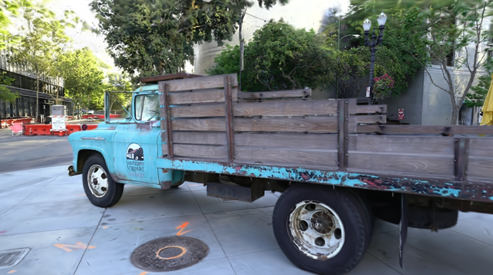
Tanks & Temples truck (428k Gaussians) rendered by the fast path — 45.5 dB PSNR against the training rasterizer, at 2× the frame rate.

Usage

from mlx3d.splatting import FastGaussianRenderer, GaussianModel

model = GaussianModel.load_ply("point_cloud.ply")
renderer = FastGaussianRenderer(model)       # caches activations, covariances, SH
out = renderer.render(camera)                # {"image", "alpha"}

Everything is also reachable from the CLI:

mlx3d-view point_cloud.ply --fast            # interactive viewer, fast RGB frames
mlx3d-render point_cloud.ply --fast --out render.png
python examples/benchmark_fast_rasterization.py --ply point_cloud.ply

One-shot functional form (mirrors render_gaussians, no cross-frame caching):

from mlx3d.splatting import render_gaussians_fast

out = render_gaussians_fast(camera, means, quats, scales_act, opacities_act, sh=sh)

Useful knobs on the class:

• sh_degree=0..3 — cap the evaluated spherical-harmonic degree (0 is fastest, view-independent color).
• t_min — early-termination transmittance. The default 1/255 stops compositing as soon as no further splat could change an 8-bit pixel (training uses 1e-4).
• color_refresh — fraction of the scene radius the camera must move before view-dependent SH colors are re-evaluated (0 = every frame).
• antialias=True — Mip-Splatting opacity compensation, as in training.

Why it is faster

The training rasterizer must stay differentiable and rebuild everything every frame. The fast path exploits the fact that a viewer renders the same scene many times:

1. One fused "geometry" kernel. Camera transform, EWA projection, conics, culling, and tile bounds run in a single Metal pass per Gaussian — replacing ~60 elementwise MLX ops (~3.3 ms → 0.4 ms for 200k Gaussians).
2. Cross-frame caching. Activations (exp/sigmoid), 3D covariances, and SH-evaluated colors are computed once; colors refresh only when the camera moves enough to matter.
3. Cheaper sorting. Gaussians are depth-sorted once globally (N keys), so tile duplicates are emitted already depth-ordered and only a stable 32-bit tile-key sort remains — the training path sorts 64-bit (tile, depth) keys over every duplicate.
4. No mid-frame CPU/GPU sync. Duplicate buffers persist across frames and grow on demand, so a whole frame is submitted as one lazy graph. The training path must stall mid-frame to size its buffers.
5. Forward-only compositing. No backward bookkeeping, fp16 splat colors (conics stay fp32 — near-camera footprints underflow half precision), and an 8-bit-aware early-out.

Benchmarks

Apple M1 Pro (16 GB), macOS, MLX 0.31. Orbiting camera; mean frame latency.

Real scene — Tanks & Temples truck (428k Gaussians, SH 3)

viewpoint set	resolution	reference	fast	speedup	PSNR
dataset cameras	979×546	63.9 ms (15.6 fps)	30.8 ms (32.4 fps)	2.07×	45–49 dB
dataset cameras	1958×1092	193.8 ms (5.2 fps)	96.4 ms (10.4 fps)	2.01×	45–49 dB

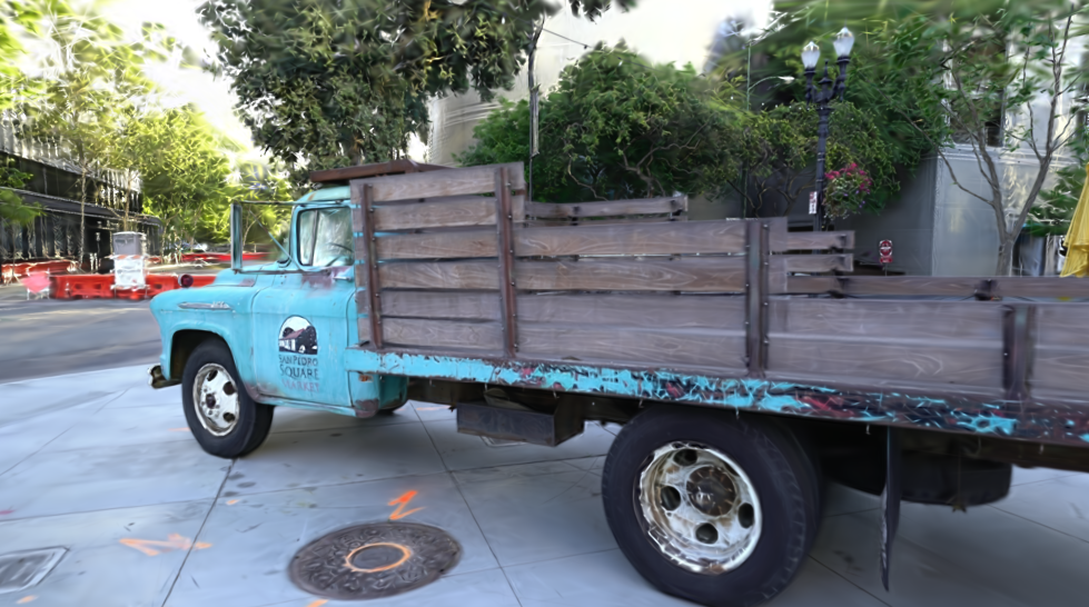
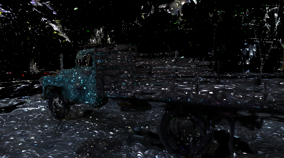
Left: training rasterizer. Right: |difference| of the two paths amplified 50× — the residual is fp16 color quantization noise.

Synthetic scenes

scene	resolution	reference	fast	speedup
50k Gaussians	1280×720	10.3 ms (97 fps)	7.0 ms (143 fps)	1.48×
200k Gaussians	1280×720	34.6 ms (29 fps)	20.6 ms (49 fps)	1.68×
500k Gaussians	1280×720	75.8 ms (13 fps)	37.2 ms (27 fps)	2.04×
500k Gaussians	1920×1080	131.5 ms (7.6 fps)	62.2 ms (16 fps)	2.11×
20k large splats	1920×1080	237.7 ms (4.2 fps)	63.9 ms (16 fps)	3.72×

The advantage grows with the pixel-to-point ratio (large splats, high resolution) — the same regime the original CUDA implementation highlights.

Dynamic (4D) sequences

Because covariances, colors, and buffers are owned by the renderer, update() makes per-timestep playback cheap. The Dynamic 3D Gaussians juggle sequence (336k Gaussians × 150 timesteps, per-timestep positions, rotations, and colors):

renderer = FastGaussianRenderer(**sequence.timestep(0))
for t in range(sequence.num_timesteps):
    renderer.update(**sequence.timestep(t))     # new means/quats/colors
    frame = renderer.render(camera)["image"]

playback (640×360, orbiting)	ms / frame	fps
reference render_gaussians	25.1	39.8
fast (update + render)	14.9	67.3

The full juggle sequence — every timestep's positions, rotations, and colors streamed through update() and rendered entirely by the fast path (67 fps at 640×360, ~14 fps at the 960×540 shown here, on an M1 Pro).

Timesteps 0 / 60 / 120 of the orbit.

See examples/play_dynamic_gaussians.py for the full loader (including how to fetch one scene of the release without downloading the whole 11.5 GB archive).

Limitations

• Forward-only. No gradients flow through FastGaussianRenderer; use render_gaussians for training and losses.
• EWA pinhole projection only (no projection="ut" distortion-aware mode).
• Splat colors are quantized to fp16 (worst-case ~0.1% per channel); if you need bit-exact output for evaluation metrics, render with the training path.
• Stale-color rendering (color_refresh > 0) is an approximation while the camera moves; set color_refresh=0 for exact view-dependent color every frame.