NeRF: Neural Radiance Fields

Train a NeRF on the Blender synthetic scenes, natively on your Mac's GPU. Full script: examples/train_nerf.py.

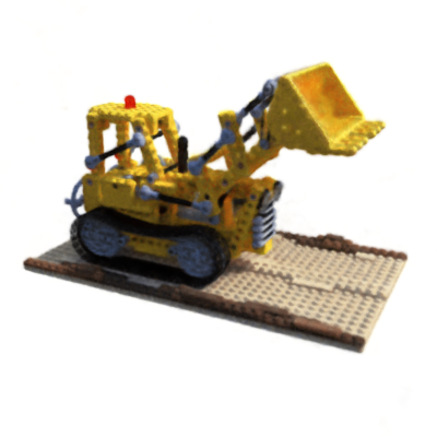
Lego scene rendered from the MLX3D hash-grid NeRF example output.

Background

A NeRF represents a scene as a function \( (x, d) \mapsto (\sigma, c) \): an MLP maps a 3D position and view direction to volume density and color. Images are formed by sampling points along camera rays and compositing with the volume rendering quadrature

\[ C = \sum_i T_i\, (1 - e^{-\sigma_i \delta_i})\, c_i, \qquad T_i = e^{-\sum_{j<i} \sigma_j \delta_j}. \]

MLX3D provides each piece as a separate, reusable function.

Data

Download the NeRF synthetic dataset (e.g. the lego scene). Then:

from mlx3d.datasets import load_blender

train = load_blender("nerf_synthetic/lego", "train", downscale=4)
camera, image = train[0]   # Camera, (H, W, 3) image

The loader converts Blender's OpenGL-style camera matrices to MLX3D's OpenCV convention and composites the RGBA renders onto white.

Rays

Every pixel of every training view becomes one ray:

import mlx.core as mx

all_o, all_d, all_c = [], [], []
for cam, img in zip(train.cameras, train.images):
    o, d = cam.generate_rays()           # (H, W, 3) each
    all_o.append(o.reshape(-1, 3))
    all_d.append(d.reshape(-1, 3))
    all_c.append(img.reshape(-1, 3))
origins, dirs, colors = (mx.concatenate(x) for x in (all_o, all_d, all_c))

Model and rendering

render_rays runs the full pipeline: stratified coarse sampling, the MLP, optional hierarchical (importance) fine sampling, and volume rendering.

from mlx3d.nn import NeRF, render_rays

model = NeRF()  # 8x256 MLP, 10/4 positional encoding frequencies

out = render_rays(
    model, origins[:1024], dirs[:1024],
    near=2.0, far=6.0,
    num_coarse=64, num_fine=64,
    white_background=True,
)
out["rgb"]    # (1024, 3)
out["depth"]  # (1024,)

Training loop

import mlx.nn as nn
import mlx.optimizers as optim
import numpy as np

optimizer = optim.Adam(learning_rate=5e-4)

def loss_fn(model, o, d, c):
    out = render_rays(model, o, d, 2.0, 6.0, num_coarse=64, num_fine=64,
                      white_background=True)
    loss = ((out["rgb"] - c) ** 2).mean()
    if "rgb_coarse" in out:                       # supervise both passes
        loss = loss + ((out["rgb_coarse"] - c) ** 2).mean()
    return loss

loss_and_grad = nn.value_and_grad(model, loss_fn)

for it in range(20_000):
    idx = mx.array(np.random.randint(0, origins.shape[0], (1024,)))
    loss, grads = loss_and_grad(model, origins[idx], dirs[idx], colors[idx])
    optimizer.update(model, grads)
    mx.eval(model.parameters(), optimizer.state)

Or simply run the script:

python examples/train_nerf.py --data nerf_synthetic/lego --downscale 4

Performance

• Render evaluation images in chunks (the script uses 4096 rays) to bound memory.
• mx.eval once per step; never call .item() inside the loop.
• The original NeRF takes ~100k+ iterations for full quality; at --downscale 4 you will see a recognizable scene within a few thousand iterations.

For real-time-renderable scenes trained in minutes rather than hours, continue to Gaussian Splatting.