Mesh Rendering and Extraction

MLX3D includes a differentiable soft mesh rasterizer for optimization loops, UV texture rendering for OBJ assets, and scalar-field mesh extraction.

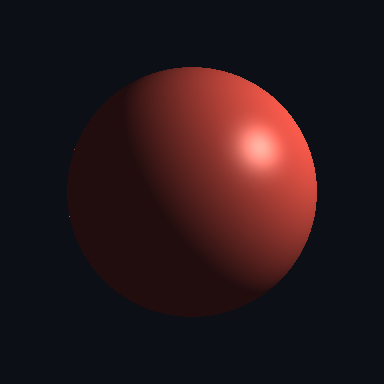
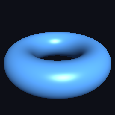
Material and lighting previews rendered by MLX3D's hard mesh rasterizer and shader stack.

Soft Rasterization

render_mesh_soft projects triangles through an MLX3D camera and blends them with SoftRas-style coverage and depth weighting. The renderer is written in MLX, so gradients flow to vertices, colors, and texture values.

import mlx.core as mx
from mlx3d.cameras import Camera
from mlx3d.renderer import render_mesh_soft

cam = Camera.look_at(eye=(0, 0, -3), at=(0, 0, 0), width=256, height=256)
verts = mx.array([[-0.7, -0.6, 0.0], [0.7, -0.6, 0.0], [0.0, 0.7, 0.0]])
faces = mx.array([[0, 1, 2]], dtype=mx.int32)
face_colors = mx.array([[0.1, 0.8, 1.0]])

out = render_mesh_soft(cam, verts, faces, face_colors=face_colors, sigma=0.02)
image = out["image"]
alpha = out["alpha"]

Use small sigma values for sharper silhouettes and larger values for smoother optimization gradients. This renderer targets differentiable losses and medium-resolution previews; Gaussian Splatting remains the real-time viewer path for large splat scenes.

Textured OBJ Rendering

load_obj parses mtllib and common diffuse map_Kd textures. The returned ObjData contains texcoords, faces_texcoords_idx, and texture_image when they are present.

from mlx3d.io import load_obj
from mlx3d.renderer import render_mesh_soft

obj = load_obj("asset.obj")
out = render_mesh_soft(
    cam,
    obj.verts,
    obj.faces,
    texcoords=obj.texcoords,
    faces_texcoords_idx=obj.faces_texcoords_idx,
    texture=obj.texture_image,
)

MLX3D uses OBJ UV convention for sampling: v=0 is the bottom of the image.

Textured glTF / GLB Assets

In 0.2.0, glTF loading covers default-scene nodes, triangle primitives, node transforms, UVs, material IDs, PBR base-color factors, metallic/roughness factors, and base-color textures from data URIs, external images, or GLB bufferViews. save_gltf(..., texture_image=...) writes a self-contained GLB with an embedded PNG texture, which is useful for portable examples and asset previews.

from mlx3d.io import load_gltf
from mlx3d.renderer import render_mesh
from mlx3d.structures import Meshes

asset = load_gltf("textured_asset.glb")
mesh = Meshes([asset.verts], [asset.faces])

out = render_mesh(
    cam,
    mesh,
    texture=asset.texture_image,
    verts_uvs=asset.uvs,
    faces_uvs=asset.faces,
    shading="pbr",
    roughness=asset.materials[0].roughness_factor,
    metallic=asset.materials[0].metallic_factor,
)

Mesh Extraction

marching_cubes extracts a mesh from a scalar grid and returns a Meshes object. Internally it uses a marching-tetrahedra cube decomposition, which avoids ambiguous cube cases while keeping the familiar marching-cubes API.

import numpy as np
import mlx.core as mx
from mlx3d.ops import marching_cubes

xs = np.linspace(-1, 1, 64)
z, y, x = np.meshgrid(xs, xs, xs, indexing="ij")
sdf = x * x + y * y + z * z - 0.5

mesh = marching_cubes(
    mx.array(sdf),
    level=0.0,
    spacing=(2 / 63, 2 / 63, 2 / 63),
    origin=(-1, -1, -1),
)
print(mesh.verts_packed().shape, mesh.faces_packed().shape)

Signed Distance Functions

For procedural shapes you usually do not have a grid in hand — you have a function. The sdf_* helpers in mlx3d.ops give analytic primitives (sdf_sphere, sdf_box, sdf_torus, sdf_plane) and constructive-solid-geometry operators (sdf_union, sdf_intersection, sdf_difference, and their smooth sdf_smooth_* variants) that compose with plain function calls. sdf_to_mesh samples such a function on a grid and runs marching cubes for you:

import mlx.core as mx
from mlx3d.ops import sdf_box, sdf_sphere, sdf_smooth_difference, sdf_to_mesh

def model(p: mx.array) -> mx.array:
    cube = sdf_box(p, half_extents=(0.6, 0.6, 0.6))
    bite = sdf_sphere(p, radius=0.78, center=(0.55, 0.55, 0.55))
    return sdf_smooth_difference(cube, bite, k=0.15)

mesh = sdf_to_mesh(model, resolution=96, bounds=1.4)

Because the primitives and operators are pure MLX, the field is differentiable w.r.t. its parameters (radii, centers, ...), so the same helpers double as a loss for SDF shape fitting. See examples/sdf_csg.py for a full CSG-to-render walkthrough.